1.0.1 Specifications
Develop a model to meet the data points for tire slip in icy and wet conditions. The Pacejka model will be used and for different conditions, the model parameters will be found.
\[\mu(\kappa)=c_1\left[1-e^{-c_2\kappa}\right]-c_3\kappa\]1.0.2 Data
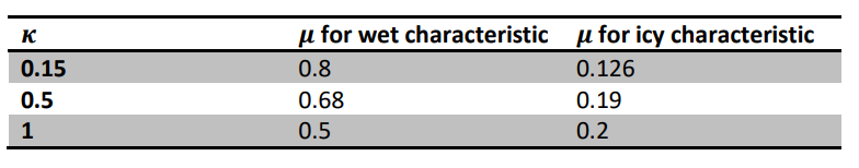
For icy and wet road conditions, the following information was determined experimentally.
1.0.3 Parameters
| Parameters | Wet | Icy |
|---|---|---|
| c1 | 0.86 | 0.2 |
| c2 | 33.078 | 6.628 |
| c3 | 0.36 | 0 |
1.1.0 Method of Finding Parameters
Use the fact that the linear part is asymptote of the function so the slope and intercept gives us c1 and c3.
Then you plug in values to find c2
1.1.1 Programs for Pacejka Model
After the model parameters are found, they can be implemented into a Simulink model as shown.
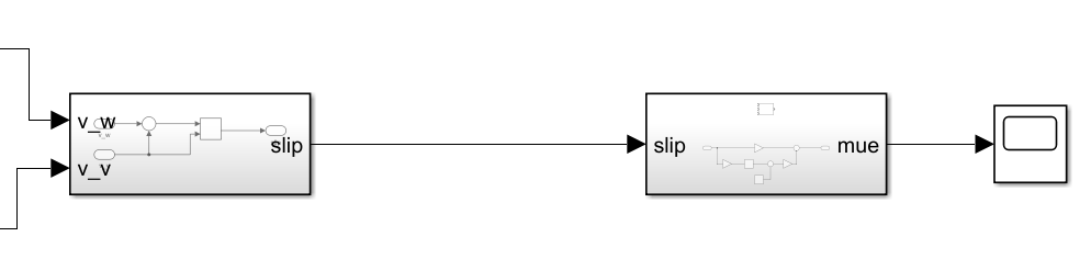
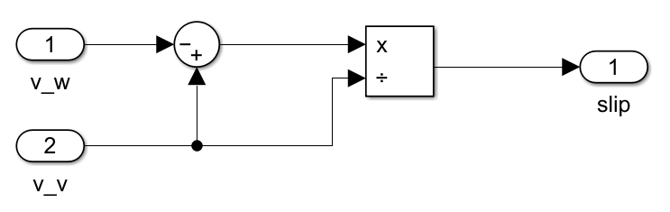
Simulink Model for slip calculation
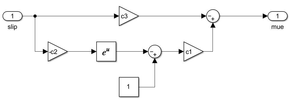
Simulink Model for
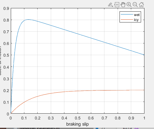
To observe the relationship between friction coefficient and slip, we also implemented a simple Matlab script to plot the graph.
%% Setup
% Wet
c1w=86/100;
c2w=33078/1000;
c3w=36/100;
f_mue_w = @(x)(c1w*(1-exp(-c2w*x))-c3w*x);
% Icy
c1i=2/10;
c2i=6628/1000;
c3i=0;
f_mue_i = @(x)(c1i*(1-exp(-c2i*x))-c3i*x);

%% Ploting friction against slip in different road conditions
fplot(f_mue_w,[0,1])
hold on
fplot(f_mue_i,[0,1])
hold off
grid
legend('wet','icy')
xlabel('braking slip')
ylabel('coef. of friction')
ylim([0 0.9])
1.1.2 Extension of Model for Parameterization
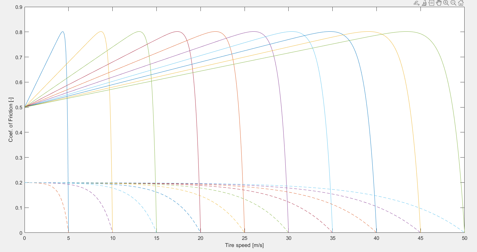
To see how the friction coefficient varies with different speeds of the vehicle or tires, we extended the models.
%% Ploting friction against tire speed in different road conditions and vehicle velocities (braking)
f_slip = @(v_v,v_w)((v_v-v_w)/(v_v));
for i=5:5:50
slip_val = f_slip(i,0:0.1:i);
plot(0:0.1:i,f_mue_w(slip_val),"-")
hold on
plot(0:0.1:i,f_mue_i(slip_val),"--")
end
xlabel('Tire speed [m/s]'); ylabel('Coef. of Friction [-]')
hold off
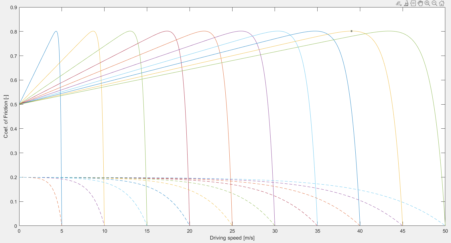
%% Ploting friction against driving speed in different road conditions and tire velocities (accelerating)
f_slip = @(v_w,v_v)((v_w-v_v)/(v_w));
for i=5:5:50
slip_val = f_slip(i,0:0.1:i);
plot(0:0.1:i,f_mue_w(slip_val),"-")
hold on
plot(0:0.1:i,f_mue_i(slip_val),"--")
end
xlabel('Tire speed [m/s]'); ylabel('Coef. of Friction [-]')
hold off
1.2.0 Results for Model Parameters
| Parameters | Wet | Icy |
|---|---|---|
| c1 | 0.86 | 0.2 |
| c2 | 33.078 | 6.628 |
| c3 | 0.36 | 0 |
1.2.1 Friction Slip Relationship Results
1.2.2 Rudimentary Observations from Model
| v_v | v_w | mue |
|---|---|---|
| 40 | 38 | 0.68 |
| 30 | 28 | 0.74 |
| 30 | 22 | 0.76 |
| 40 | 22 | 0.7 |
| 60 | 22 | 0.63 |
| 30 | 30 | 0 |
| 30 | 32 | -7 |
| 15 | 10 | 0.74 |
| 15 | 5 | 0.62 |
| 15 | 14 | 0.74 |
| 100 | 15 | 0.56 |
| 100 | 80 | 0.79 |
| 100 | 90 | 0.79 |
| 100 | 99 | 0.24 |
| 100 | 50 | 0.68 |
1.2.3 General Graphs from Extended Model